ACM_BCB
Module 2: Epigenetic Clock Analysis
How Old Are You Really? From DNA Methylation to Biological Age
A Hands-On Workshop
Workshop Overview
This hands-on tutorial walks through four activities: **This tutorial requires R and R studio and has been tested on R4.5 and R4.6.** **Please download the [R markdown file and required data zipped file](https://github.com/kobor-lab/ACM_BCB/blob/main/Epigenetic_clock_analysis_zip.zip))** and unzip the files. This directory contain the script [Epigenetic_clock_analysis_RMD.Rmd](https://github.com/kobor-lab/ACM_BCB/blob/main/Epigenetic_clock_analysis_RMD.Rmd) and the data files for running the script.
- Activity 1 — DNA methylation exploration and PCA
- Activity 2 — Calculation of epigenetic clocks
- Activity 3 — Computation and visualization of Epigenetic Age Difference (EAD) and Epigenetic Age Acceleration (EAA)
- Activity 4 — Association analyses linking EAA to health-related variables, including Adults with Congenital Heart Disease (ACHD) surgery status with and without Age or cell-type correction
What’s Covered
- PCA of whole blood DNA methylation beta values
- Epigenetic clock calculation (1st, 2nd, and 3rd generation)
- EAD and EAA derivation and visualization
- Robust linear regression for association testing
- Cell-type correction strategies
Out of Scope
- DNAm QC & preprocessing — see Zhuang & Jude et al. 2025 and the EPICv2 QC pipeline; also Konwar et al. 2021 and the DNAm QC and preprocessing pipeline
- Cell-type deconvolution of 12 immune cell types by Salas et al. 2022
Setup: R Packages
Install required packages
# # Run once to install all required packages
packages <- c(
  "knitr",
  "dplyr",
  "tidyr",
  "reshape2",
  "table1",
  "broom",
  "ggplot2",
  "ggpubr",
  "patchwork",
  "pheatmap",
  "MASS",
  "sfsmisc",
  "robustbase"
)

install.packages(packages)

# Bioconductor packages
if (!require("BiocManager", quietly = TRUE))
  install.packages("BiocManager")

# methylCIPHER and DunedinPACE are GitHub packages
if (!require("remotes", quietly = TRUE))
  install.packages("remotes")

remotes::install_github("HigginsChenLab/methylCIPHER")
remotes::install_github("danbelsky/DunedinPACE")


BiocManager::install("preprocessCore") # for DunedinPACE
Load libraries and helper functions
library(knitr)
library(dplyr)
library(tidyr)
library(reshape2)
library(table1)
library(broom)
library(methylCIPHER)
library(ggplot2)
library(ggpubr)
library(patchwork)
library(DunedinPACE)
library(pheatmap)
library(MASS)
library(sfsmisc)
library(robustbase)

dir.create("results")
# for PCA loading and variable association tests
wrapperPlotPCAR2 <- function(Loadings, Importance,
                                meta_categorical = NULL,
                                meta_continuous  = NULL,
                                P_threshold      = 0.05,
                                p_title          = "",
                                geom.text.size   = 3,
                                round_digit      = 3,
                                show_legend      = TRUE,
                                multiple_test_correction = TRUE) {

  library(broom)
  library(dplyr)
  library(ggplot2)

  # --- Helper: ANOVA R2 ---
  get_anova_r2 <- function(pc_idx, covar_name) {
    fit   <- aov(Loadings[, pc_idx] ~ meta_categorical[, covar_name])
    fit   <- car::Anova(fit, type = "II")
    tidy_fit <- tidy(fit)

    ss_reg <- tidy_fit$sumsq[1]
    ss_res <- tidy_fit$sumsq[2]

    data.frame(
      term      = covar_name,
      statistic = tidy_fit$statistic[1],
      PC        = paste0("PC", pc_idx),
      R_squared = ss_reg / (ss_reg + ss_res),
      p.value   = tidy_fit$p.value[1],
      Variation = get_variation(pc_idx),
      method    = "ANOVA"
    )
  }

  # --- Helper: Correlation R2 ---
  get_cor_r2 <- function(pc_idx, covar_name) {
    fit <- cor.test(Loadings[, pc_idx], meta_continuous[, covar_name],
                    method = "pearson", alternative = "two.sided")
    data.frame(
      term      = covar_name,
      statistic = fit$statistic,
      PC        = paste0("PC", pc_idx),
      R_squared = fit$estimate^2,
      p.value   = fit$p.value,
      Variation = get_variation(pc_idx),
      method    = "Pearson's product-moment correlation"
    )
  }

  # --- Helper: get % variance for a PC ---
  get_variation <- function(pc_idx) {
    round(Importance[pc_idx] * 100, 2)
  }

  # --- Run tests ---
  results_cat  <- if (!is.null(meta_categorical)) {
    do.call(rbind, lapply(1:ncol(Loadings), function(i)
      do.call(rbind, lapply(colnames(meta_categorical), function(cv) get_anova_r2(i, cv)))))
  }

  results_cont <- if (!is.null(meta_continuous)) {
    do.call(rbind, lapply(1:ncol(Loadings), function(i)
      do.call(rbind, lapply(colnames(meta_continuous), function(cv) get_cor_r2(i, cv)))))
  }

  # --- Combine results ---
  all_results <- rbind(results_cat, results_cont)
  all_results$adjP <- p.adjust(all_results$p.value, method = "bonferroni")

  variable_level <- rev(c(colnames(meta_categorical), colnames(meta_continuous)))

  # --- Significance label ---
  legend_title <- ifelse(multiple_test_correction, "Adjusted p", "Nominal p")
  all_results <- all_results %>%
    mutate(sig_color = ifelse(
      (if (multiple_test_correction) adjP else p.value) <= P_threshold,
      paste0("<=", P_threshold), paste0(">", P_threshold)
    ))

  # --- PC axis labels with % variance ---
  all_results$PC <- factor(all_results$PC)
  all_results$term <- factor(all_results$term, levels = variable_level)

  pc_var <- all_results %>% dplyr::select(PC, Variation) %>% distinct()
  levels(all_results$PC) <- paste0(pc_var$PC, "\n(", pc_var$Variation, "%)")

  # --- Color scale for significant associations---
  sig_colors <- setNames(
    c("#ffc4c4", "lightgrey"),
    c(paste0("<=", P_threshold), paste0(">", P_threshold))
  )

  # --- Plot ---
  p <- ggplot(all_results, aes(PC, term, fill = sig_color)) +
    geom_tile(color = "white") +
    geom_text(aes(label = round(R_squared, round_digit)), size = geom.text.size) +
    scale_fill_manual(values = sig_colors) +
    coord_fixed() +
    ggtitle(p_title) +
    guides(fill = guide_legend(title = legend_title)) +
    theme_minimal() +
    theme(
      panel.grid  = element_blank(),
      axis.title  = element_blank(),
      axis.ticks.y = element_blank()
    )

  if (!show_legend) p <- p + theme(legend.position = "none")

  return(list(plot = p, stats = all_results))
}


# plot Age vs. clock and Calculate Median Absolute Error
plotClockMdAE <- function(SampleInfo, clock_i){
  SampleInfo$EpiAge <- SampleInfo[, clock_i]

  mae_val <- median(abs(SampleInfo$EpiAge - SampleInfo$Age)) #median absolute error between clock and chronological age

  # Scatter plot
  ggplot(SampleInfo, aes(x = Age, y = EpiAge)) +
    geom_point(alpha = 0.6, color = "steelblue") +
    geom_smooth(method = "lm", se = TRUE, color = "red", fill = "lightpink") +
    geom_abline(slope = 1, intercept = 0, linetype = "dashed", color = "gray40") +
    stat_cor(method = "pearson", label.x.npc = "left", label.y.npc = "top") +
    annotate(
      "text",
      x = Inf, y = -Inf,
      hjust = 1.1, vjust = -1,
      label = paste0("Median Absolute Error = ", round(mae_val, 2), " years"),
      fontface = "italic",
      size = 4,
      color = "gray20"
    ) +
    labs(
      title = paste0("Chronological Age vs " ,clock_i),
      x     = "Chronological Age (years)",
      y     = "Epigenetic Age (years)"
    ) +
    theme_classic()
}
Activity 1: PCA of DNA Methylation Beta Values
Goal
Apply Principal Component Analysis (PCA) to whole blood DNA methylation beta values to identify the primary biological drivers of DNA methylation variantion, such as chronological age, sex, and estimated immune cell-type proportions. </div>
This activity uses a subset of samples and CpGs from dataset GSE286313 (from Zhuang & Jude et al. 2025). The CpG subset contains clock probes used to calculate the Horvath Pan-Tissue, Hannum, PhenoAge, GrimAge, and DunedinPACE clocks.
Load beta value and Sample metadata
The provided beta matrix has been preprocessed (background correction, functional normalization, batch correction for technical batches (Chip ID and Chip position))
SampleInfo <- readRDS("data/SampleInfo_n44_VHAS_CALERIE.rds")
beta_matrix <- readRDS("data/matrix_x_clock_probes_n44.rds")
dim(beta_matrix) # 41353    44
Explore data
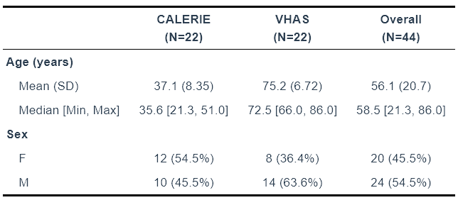
Sample demographics
df <- SampleInfo
df$Sex    <- factor(df$Sex)
df$Cohort <- factor(df$Cohort)

# Optional: add labels
label(df$Age)    <- "Age (years)"
label(df$Sex)    <- "Sex"
label(df$Cohort) <- "Cohort"

# Create Table 1
table1(~ Age + Sex|Cohort, data = df)
DNA methylation beta value density
Beta_sample_melted<- reshape2::melt(beta_matrix)

Beta_Plot<-Beta_sample_melted[which(Beta_sample_melted$value >= 0),]
colnames(Beta_Plot)[2:3] <- c("Sample_Name", "Beta_Value")

# plot the density
ggplot(Beta_Plot, aes_string("Beta_Value", group="Sample_Name",label = "Sample_Name"))+
  geom_density(size=0.2, alpha = 0.5)+
  theme_bw()+
    labs(
    title = "DNA Methylation density (selected clock probes = 41353)",
    x     = "DNAm beta value"
  )
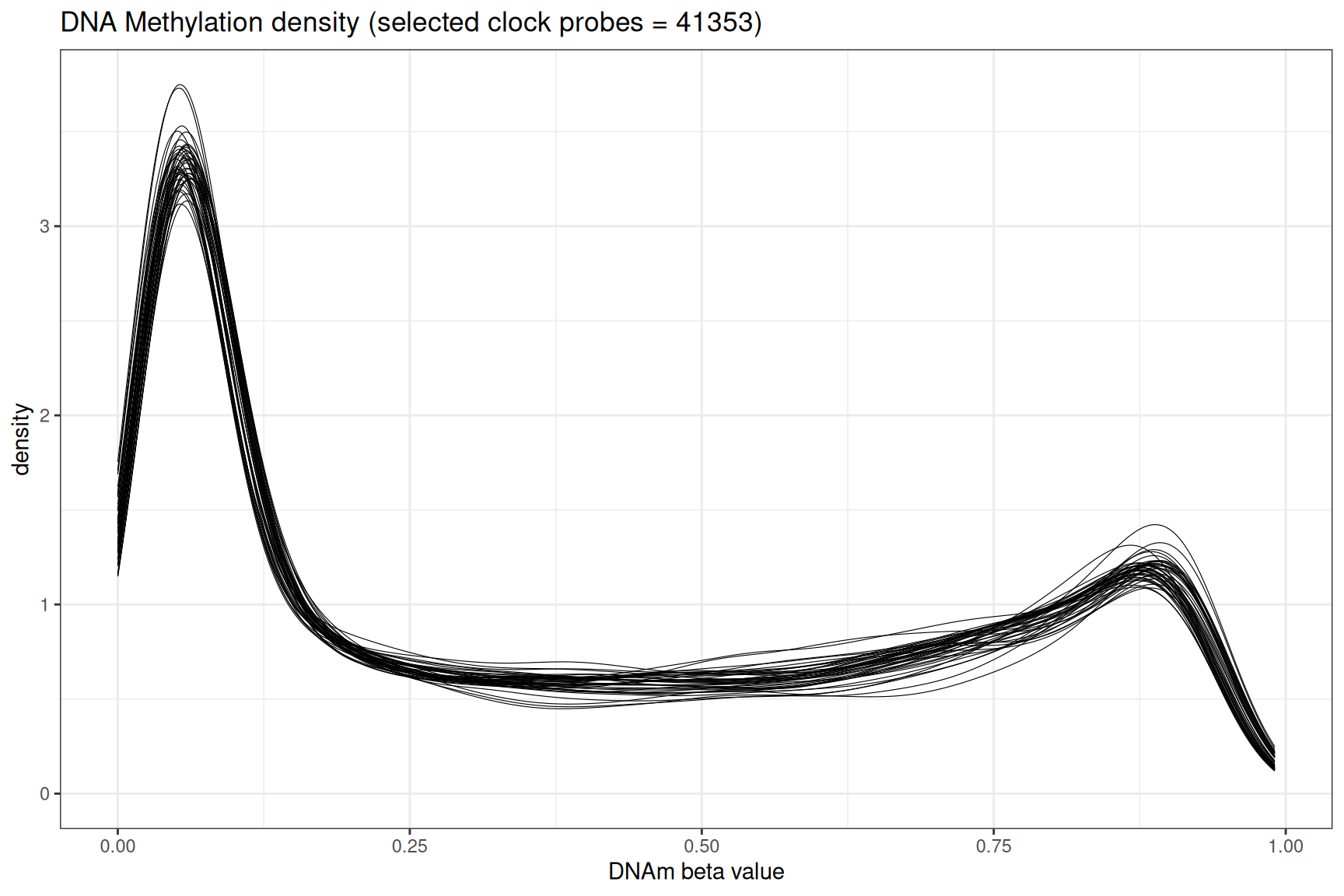
Key takeaway: The bimodal distribution: with a peak near 0 (fully unmethylated) and near 1 (fully methylated),is expected in whole blood DNA methylation profiles.
Principal Component Analysis
PCA analysis
sexProbeIDs <- readRDS("data/sexProbeIDs.rds") # there are 886 probes mapped to Chr X or Y in these 41353 probes. Remove sex probes before running PCA
betas <- beta_matrix[!(rownames(beta_matrix)%in%rownames(sexProbeIDs)), ]
# PCA
PCA_full<-princomp(na.omit(betas))
Loadings<-as.data.frame(unclass(PCA_full$loadings))
vars <- PCA_full$sdev^2
Importance<-vars/sum(vars)
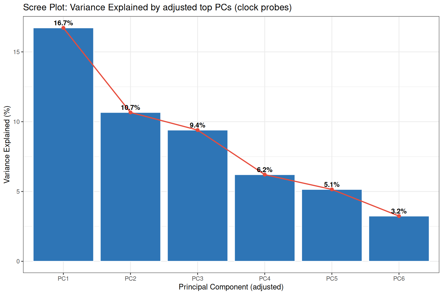
paste0(round(Importance*100, 2)[1:7], "%") #print the variance accounted for the top PCs
The top PC (PC0) accounted for 97.65% of the total variance, is dropped because it mainly represent the bi-modal distribution of the beta value, the rest of PCs are re-calibrated
### PCA ANOVA and correlation tests and plots----
f_prefix <- "PCA_anova_correlation"
p_title <- "R2 of top PCs and variable associations \n(clock probes)"
f_out_p <- paste0("results/",f_prefix, ".png")

PC_view_num <- 7 # this number included PC0, however, PC0 is not included in the association tests

#check if loading rownames are identical to Sample name
identical(rownames(Loadings), SampleInfo$Sample_Name)

# adjust importance (total variance accounted) after removing PC0
adjust<-1-Importance[1]
pca_adjusted_Importance<-Importance[2:length(Importance)]/adjust # new adjusted importance
names(pca_adjusted_Importance) <- paste0("PC", 1:length(pca_adjusted_Importance)) #must update Importance names to the new PC1
#Scree plot: variance explained per PC (PC0 removed)
tibble(
  PC              = paste0("PC", 1:6),
  VarExplained    = pca_adjusted_Importance[1:6]
) %>%
  mutate(PC = factor(PC, levels = PC)) %>%
  ggplot(aes(x = PC, y = VarExplained*100)) +
  geom_col(fill = "#2E75B6", colour = "white") +
  geom_line(aes(group = 1), colour = "#E74C3C", linewidth = 0.8) +
  geom_point(colour = "#E74C3C", size = 2) +
  theme_bw()+
    geom_text(
    aes(label = paste0(round(VarExplained * 100, 1), "%")),
    vjust = -0.5,
    fontface = "bold",
    size = 3.5
  ) +
  labs(
    title    = "Scree Plot: Variance Explained by adjusted top PCs (clock probes)",
    x        = "Principal Component (adjusted)",
    y        = "Variance Explained (%)"
  )
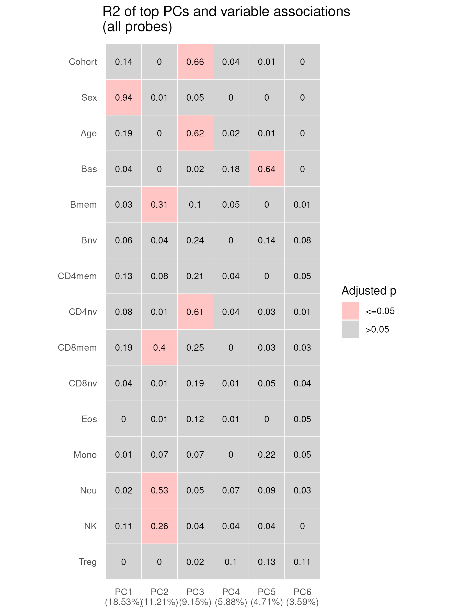
Top PCs and association with variables and predicted cell-type proportions
Understand the main drivers of variation of the DNA methylation data.
meta_categorical <- SampleInfo %>% dplyr::select(Cohort,Sex)
meta_continuous <- SampleInfo %>% dplyr::select(Age,
                                         Bas, Bmem, Bnv, CD4mem, CD4nv, # DNA methylation predicted cell types
                                         CD8mem, CD8nv, Eos, Mono, Neu,
                                         NK, Treg)


pca_df<-data.frame(adjusted_variance=pca_adjusted_Importance, PC=seq(1:length(pca_adjusted_Importance)))

Loadings_association <- Loadings[, 2:PC_view_num] # remove PC0 loading, show PC1-PC_view_num
# identical(Loadings_association %>% rownames(), SampleInfo$Sample_Name)


tmp <- wrapperPlotPCAR2(Loadings=Loadings_association,
                        Importance = pca_adjusted_Importance,
                        meta_categorical=meta_categorical,
                        meta_continuous = meta_continuous,
                        P_threshold = 0.05,
                        p_title=p_title,
                        geom.text.size = 3,
                        round_digit=2,
                        show_legend=T, multiple_test_correction = T)
p_PCA_association <- tmp[[1]]
adj_test_results <- tmp[[2]] # the test results

ggsave(plot = p_PCA_association, filename = paste0(f_out_p), width = 6, height = 8, dpi = 300)

Association of variables and loadings of the top 6 adjusted PCs. An overall F-test was carried out for separate simple linear regression models for each combination of PCs as dependent variable and the predictor variables: cohort, sex, age, and 12 cell-type proportions. R² is indicated in each cell; variance accounted (adjusted) per PC is shown in brackets on the x-axis. P-values are Bonferroni adjusted.
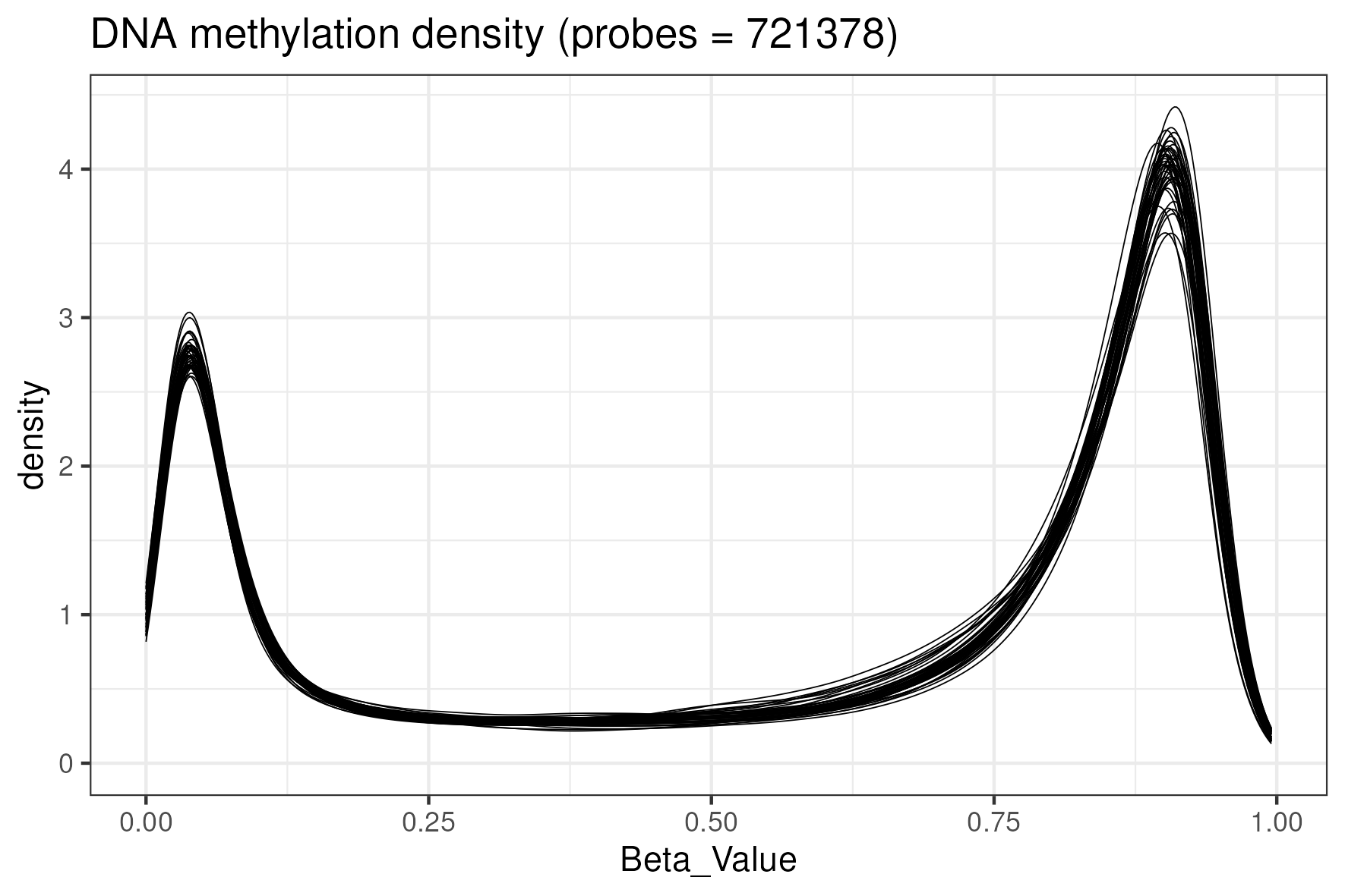
The same association tests using all array probes show a similar pattern:
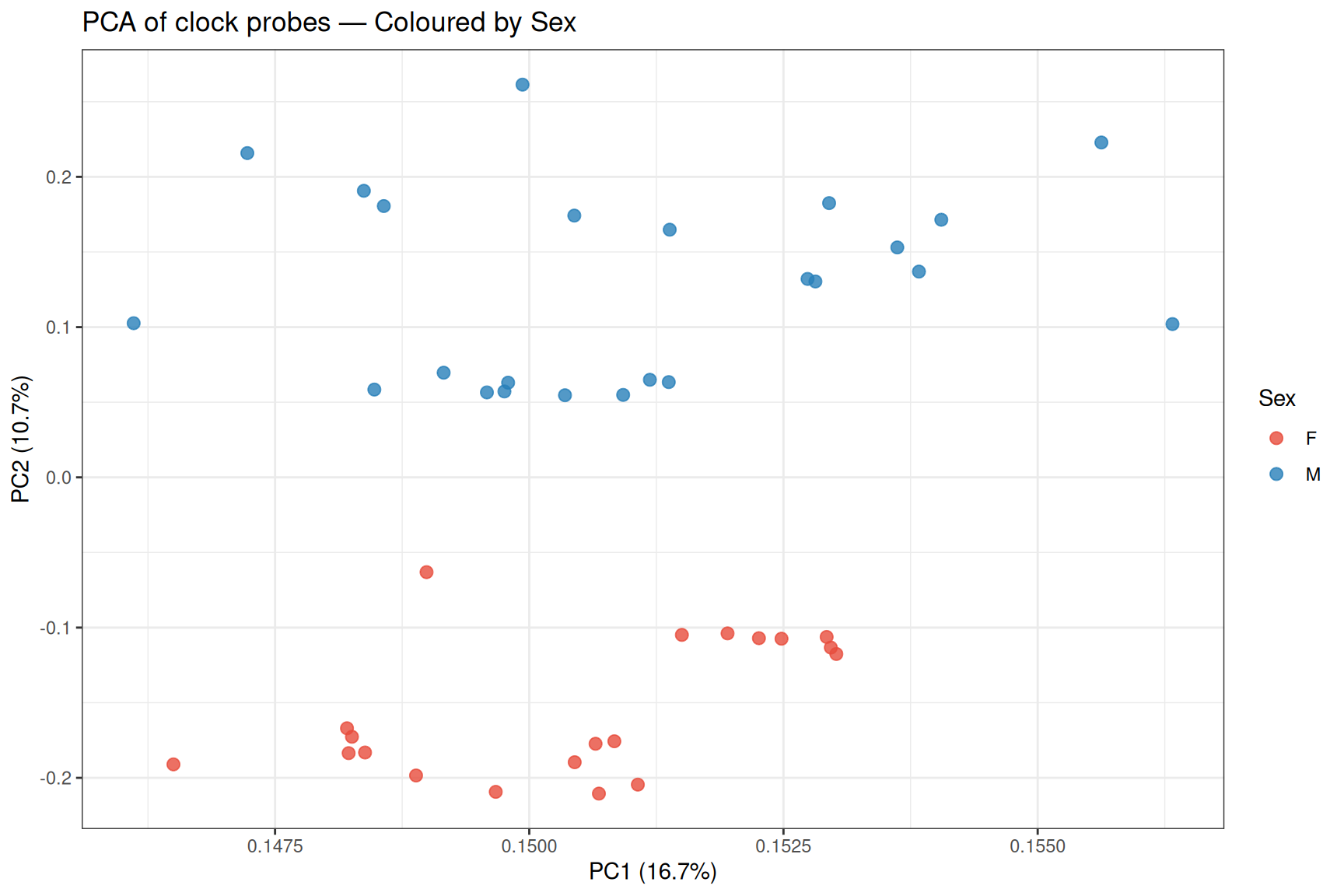
PCA scatter plots
Sex separates clearly along adjusted PC2.
# PC1 vs PC2 coloured by sex
pca_loadings <- cbind(SampleInfo, data.frame(PC1=Loadings[,1], PC2=Loadings[,2], PC3=Loadings[,3]))
p_sex <- ggplot(pca_loadings , aes(x = PC1, y = PC2, colour = Sex)) +
  geom_point(alpha = 0.8, size = 2.5) +
  scale_colour_manual(values = c("M" = "#2980B9", "F" = "#E74C3C")) +
  theme_bw()+
  labs(
    title    = "PCA of clock probes — Coloured by Sex",
    x = paste0("PC1 (", round(pca_adjusted_Importance[1]*100, 1), "%)"),
    y = paste0("PC2 (", round(pca_adjusted_Importance[2]*100, 1), "%)")
  )

p_sex
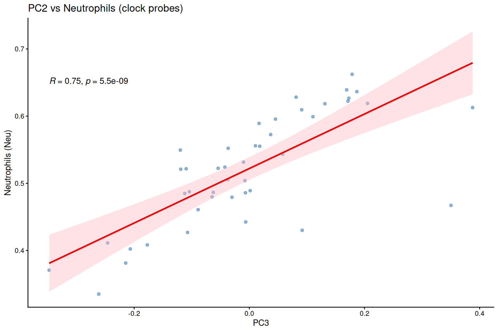
Neutrophil proportion is significantly correlated with adjusted PC3.
#PC scores vs cell-type proportions
ggplot(pca_loadings, aes(x = PC3, y = Neu)) +
  geom_point(alpha = 0.6, color = "steelblue") +
  geom_smooth(method = "lm", se = TRUE, color = "red", fill = "lightpink") +
  stat_cor(method = "pearson", label.x.npc = "left", label.y.npc = "top") +
  labs(
    title = "PC2 vs Neutrophils (clock probes)",
    y = "Neutrophils (Neu)"
  ) +
  theme_classic()
Key Takeaways — Activity 1
- Chronological age, sex, and cell-type composition are typically the main drivers of blood DNAm variation and associate with top PCs.
- Understanding these drivers is essential for correctly accounting for confounding in downstream association analyses.
</div>
Activity 2: Calculating Epigenetic Clocks with methylCIPHER
Goal
Use the methylCIPHER and DunedinPACE packages to compute a panel of established epigenetic clocks spanning first-, second-, and third-generation approaches applicable to whole blood samples. </div>
Overview of epigenetic clock generations
| Generation | Example Clocks | Trained To Predict | Training Tissue |
|---|---|---|---|
| 1st | Horvath (2013) | Chronological age | multiple tissues including blood |
| 1st | Hannum (2013) | Chronological age | Blood |
| 2nd | PhenoAge (Levine 2018) | Incorporate clinical biomarkers to predict phenotypic age | Blood |
| 2nd | GrimAge (Lu 2019) | Incorporate DNAm derived biomarkers to predict mortality (“time-to-death”) | Blood |
| 3rd | DunedinPACE (Belsky 2022) | Rate of biological aging (pace of aging) | Blood |
Calculating clocks with methylCIPHER
SampleInfo <- readRDS("data/SampleInfo_n44_VHAS_CALERIE.rds")
beta_matrix <- readRDS("data/matrix_x_clock_probes_n44.rds")
# dim(beta_matrix) # 41353    44
# ── methylCIPHER clock calculation
beta_matrix <- beta_matrix
## clean up meta for clock calculation----
clock_meta <- SampleInfo[ , c("Sample_Name", "Sex","Age")]
colnames(clock_meta) <- c("Sample_Name", "Female", "Age")
clock_meta$Female <- gsub("female", "F", clock_meta$Female, ignore.case = T)
clock_meta$Female <- (clock_meta$Female=="F")*1 # must be F=1, M=0


identical(SampleInfo$Sample_Name, colnames(beta_matrix)) # must be T

#[methylCIPHER] calculate by methylCIPHER----
beta_matrix_t <- t(beta_matrix) # row as sample, and column as cpgs


x_all <- data.frame(Sample_Name = rownames(beta_matrix_t))

predictor_ls <- c("Horvath1", "Hannum", # first generation "Horvath1" = Horvath pan-tissue
                  "PhenoAge") # second generation
Horvath_age <- calcHorvath1(DNAm = beta_matrix_t, pheno = NULL, imputation = F) #If choose imputation = T, Need to provide of named vector of CpG Imputations
Hannum_age <- calcHannum(DNAm = beta_matrix_t, pheno = NULL, imputation = F)
PhenoAge <- calcPhenoAge(DNAm = beta_matrix_t, pheno = NULL, imputation = F)
GrimAge <- calcGrimAgeV1(beta_matrix_t, clock_meta)$GrimAgeV1 #second generation
Calculating DunedinPACE
library(DunedinPACE)
DunedinPACE <- PACEProjector(betas = beta_matrix,proportionOfProbesRequired = 0.7) %>% unlist()
SampleInfo_clock <- cbind(SampleInfo, data.frame(Horvath_age = Horvath_age, Hannum_age = Hannum_age,
                                           PhenoAge=PhenoAge, GrimAge = GrimAge, DunedinPACE = DunedinPACE))
# saveRDS(SampleInfo_clock, "data/SampleInfo_n44_VHAS_CALERIE_clocks_pre_calculated.rds")
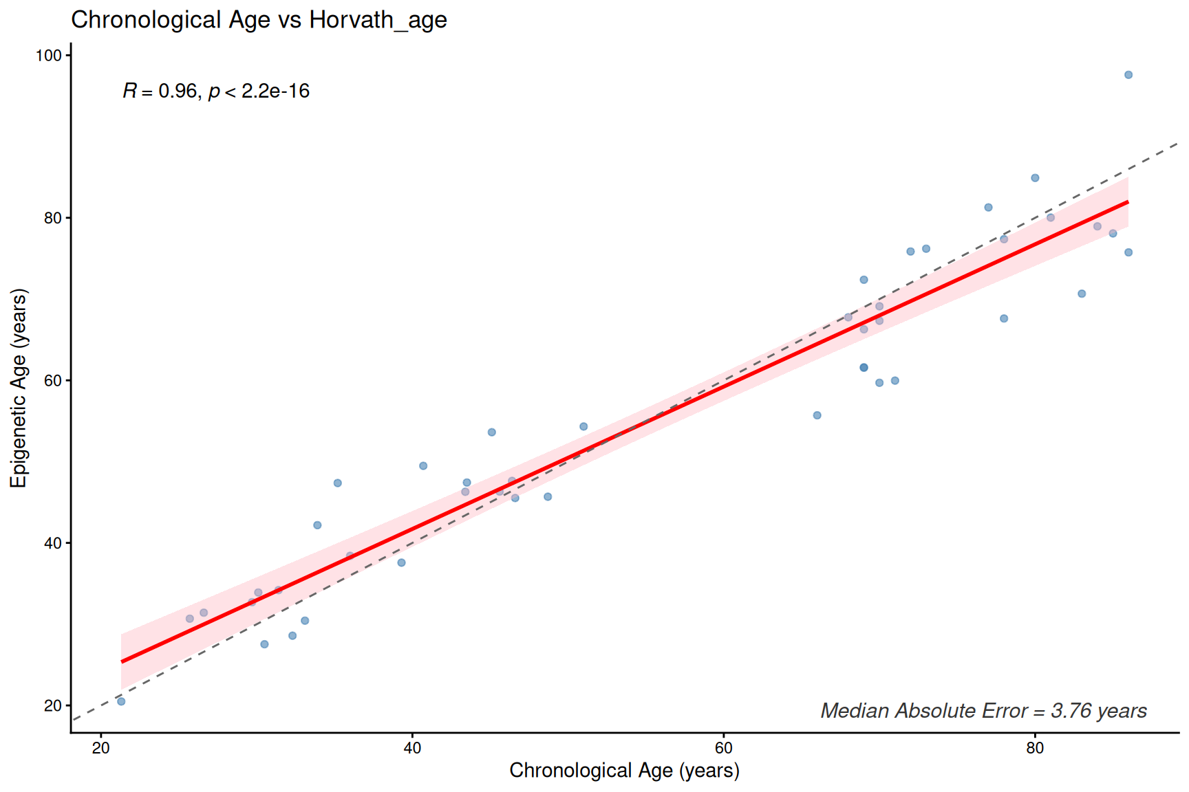
Clock and age correlation and error
SampleInfo_clock <- readRDS("data/SampleInfo_n44_VHAS_CALERIE_clocks_pre_calculated.rds")
plotClockMdAE(SampleInfo_clock, "Horvath_age")
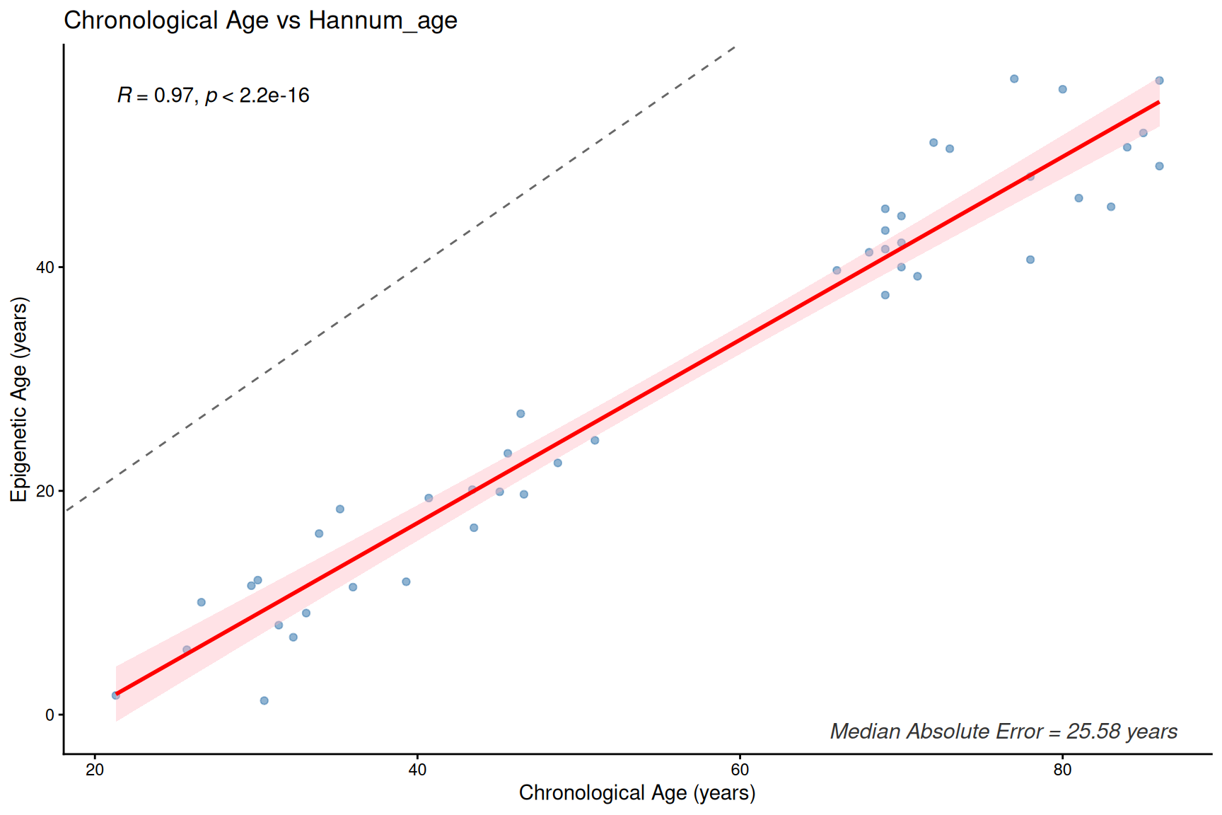
plotClockMdAE(SampleInfo_clock, "Hannum_age")
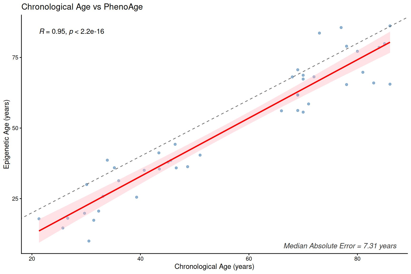
plotClockMdAE(SampleInfo_clock, "PhenoAge")
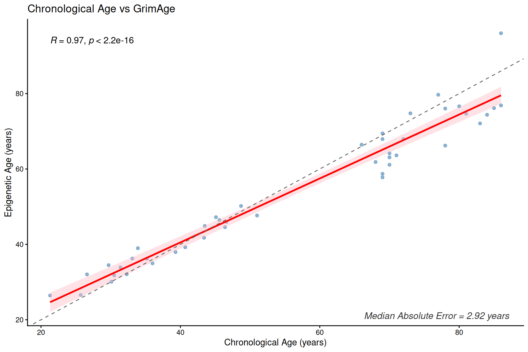
plotClockMdAE(SampleInfo_clock, "GrimAge")
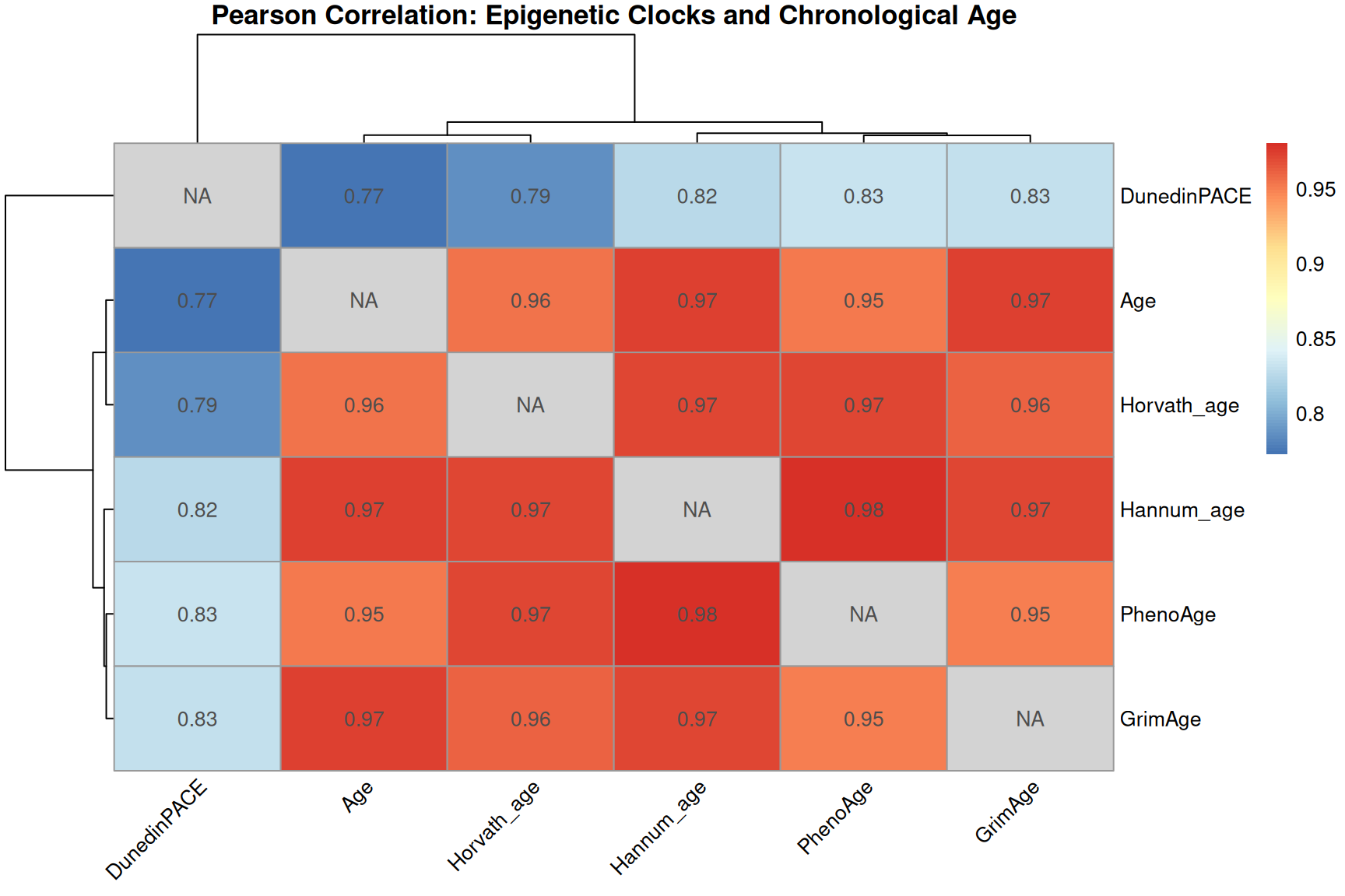
Clock and age inter-correlation heatmap
library(pheatmap)
clock_with_age <- SampleInfo_clock %>% dplyr::select(Age, Horvath_age, Hannum_age, PhenoAge, GrimAge, DunedinPACE)
row.names(clock_with_age) <- SampleInfo_clock$Sample_Name

# Compute Pearson correlation matrix
cor_mat <- cor(clock_with_age, use = "pairwise.complete.obs")
diag(cor_mat) <- NA

pheatmap(
  cor_mat,
  display_numbers = TRUE,
  number_format   = "%.2f",
  fontsize_number = 10,
  main            = "Pearson Correlation: Epigenetic Clocks and Chronological Age",
  angle_col       = 45,
  na_col          = "lightgrey",
)
Key Takeaways — Activity 2
- These first- and second-generation epigenetic clocks are expected to correlate with chronological age, but median absolute error (MdAE) varies across clocks.
- However, different clocks capture different biological constructs due to their training, especially clocks trained with health-realted information.
- DunedinPACE is a rate-based clock (units: pace of aging, not years) and should be interpreted separately from age-prediction clocks.
</div>
Activity 3: Computing Epigenetic Age Difference (EAD) and Epigenetic Age Acceleration (EAA)
Goal
Derive Epigenetic Age Difference (EAD) and Epigenetic Age Acceleration (EAA) from clock estimates. visualize both metrics and explore their inter-correlations to understand the differences between these two measures and make informed choice for downstream association analyses.
Definitions and calculations
Epigenetic Age Difference (EAD):
\[\text{EAD} = \text{Epigenetic Age} - \text{Chronological Age}\]Epigenetic Age Acceleration (EAA) — residual from a linear regression of epigenetic age on chronological age:
\(\text{Epigenetic Age}_i = \alpha + \beta \cdot \text{Chronological Age}_i + \varepsilon_i\) \(\text{EAA}_i = \varepsilon_i\)
clocks <- c("Horvath_age", "Hannum_age", "PhenoAge", "GrimAge")
eaa_names <- c("Horvath_EAA", "Hannum_EAA", "PhenoAge_EAA", "GrimAge_EAA")
ead_names <- c("Horvath_EAD", "Hannum_EAD", "PhenoAge_EAD", "GrimAge_EAD")

EAA_EDA_results <- data.frame(Sample_Name = SampleInfo_clock$Sample_Name, DunedinPACE = SampleInfo_clock$DunedinPACE)
for (i in seq_along(clocks)) {
  EAA_EDA_results[[eaa_names[i]]] <- lm(SampleInfo_clock[[clocks[i]]] ~ SampleInfo_clock$Age)$residuals # calculate EAA,sometimes also called extrinsic EAA
  EAA_EDA_results[[ead_names[i]]] <- SampleInfo_clock[[clocks[i]]] - SampleInfo_clock$Age # EAD: clock and age differences
}
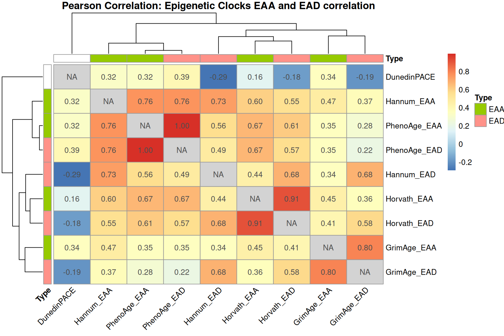
Visualize EAD, EAA, and DunedinPACE correlations
EAD and EAA generally show higher correlation within the same clock than across clocks, reflecting clock-specific methylation signatures.
row.names(EAA_EDA_results) <- EAA_EDA_results$Sample_Name
# Compute Pearson correlation matrix
cor_mat <- cor(EAA_EDA_results[,-1], use = "pairwise.complete.obs")
diag(cor_mat) <- NA

vars <- grep("EAA|EAD", colnames(EAA_EDA_results), value = T)

annotation_col <- data.frame(
  Type = ifelse(grepl("EAA", vars), "EAA", "EAD"),
  row.names = vars
)

pheatmap(
  cor_mat,
  display_numbers = TRUE,
  number_format   = "%.2f",
  fontsize_number = 10,
  main            = "Pearson Correlation: Epigenetic Clocks EAA and EAD correlation",
  angle_col       = 45,
  na_col          = "lightgrey",
  annotation_col  = annotation_col,
  annotation_row  = annotation_col
)
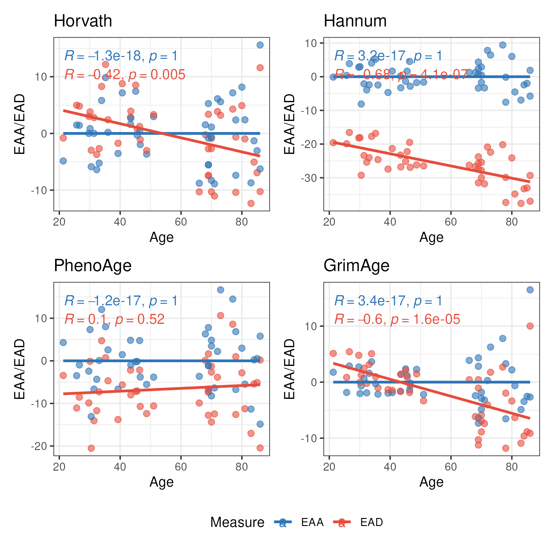
EAA, EAD vs Age
clocks <- c("Horvath", "Hannum", "PhenoAge", "GrimAge")
plot_list <- list()

for (i in seq_along(clocks)) {
  df_long <- data.frame(EAA = EAA_EDA_results[, paste0(clocks[i], c("_EAA"))],
                        EAD = EAA_EDA_results[, paste0(clocks[i], c("_EAD"))],
                        Age = SampleInfo_clock$Age) %>%
    pivot_longer(cols = c("EAA", "EAD"), names_to = "Measure", values_to = "Value")

  plot_list[[i]] <- ggplot(df_long, aes(x = Age, y = Value, colour = Measure)) +
    geom_point(alpha = 0.6, size = 2) +
    geom_smooth(method = "lm", se = FALSE) +
    stat_cor(method = "pearson", label.x.npc = "left", label.y.npc = "top") +
    scale_colour_manual(values = c(EAA = "#2E75B6", EAD = "#E74C3C")) +
    labs(
      x      = "Age",
      y      = "EAA/EAD",
      colour = "Measure",
      title  = paste0(clocks[i])
    ) +
    theme_bw()
}

# Combine with shared legend
p_EAA_EAD <- wrap_plots(plot_list, ncol = 2, guides = "collect") &
  theme(legend.position = "bottom")

ggsave(plot = p_EAA_EAD, filename = paste0("results/EAA_EAD_vs_Age.png"), width = 6, height = 6, dpi = 300)
Key Takeaways — Activity 3
- EAA is mean-zero and independent of chronological age by construction. It captures individual variation in the rate of biological aging relative to other samples in the dataset. EAA is generally more appropriate in most cases as it is robust to data preprocessing and array platform/version differences.
- EAA values are sample-set-dependent: the estimates will have to be re-calculated when the cohort composition changes (e.g. add or remove samples).
- EAD is more likely to correlate with chronological age and is more sensitive to data preprocessing and array platform/version differences.
Activity 4: Association Analyses — Biological Aging and Clinical Variables
Goal
Perform association analysis using robust linear regression to test the relationship between EAA and clinical/health-related variables. The primary exposure is ACHD surgery status (Fontan surgery vs. control), as studied in Jain & Zhuang et al. 2026. Model comparisons with and without age or cell-type correction. </div>
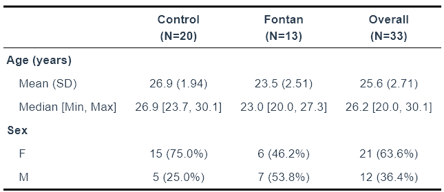
Sample demographics
SampleInfo_ACHD <- readRDS("data/SampleInfo_ACHD_n33.rds")
library(table1)
df <- SampleInfo_ACHD
df$Sex    <- factor(df$Sex)
df$surgery <- factor(df$surgery)

# Optional: add labels
label(df$Age)    <- "Age (years)"
label(df$Sex)    <- "Sex"
label(df$surgery) <- "Surgery"


# Create Table 1
table1(~ Age + Sex|surgery, data = df)
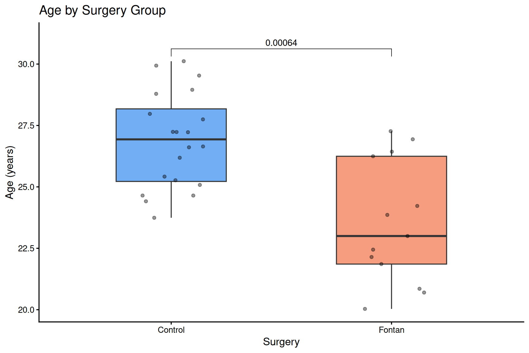
ggplot(SampleInfo_ACHD, aes(x = surgery, y = Age, fill = surgery)) +
  geom_boxplot(outlier.shape = 21, width = 0.5, alpha = 0.8) +
  geom_jitter(width = 0.15, alpha = 0.4, size = 1.5) +
  stat_compare_means(
    comparisons = list(c(levels(SampleInfo_ACHD$surgery)[1],
                         levels(SampleInfo_ACHD$surgery)[2])),
    method = "wilcox.test",
    label = "p.format"
  ) +
  scale_fill_manual(values = c("#4E9AF1", "#F4845F")) +
  scale_y_continuous(expand = expansion(mult = c(0.05, 0.10))) +
  labs(
    title = "Age by Surgery Group",
    x = "Surgery",
    y = "Age (years)"
  ) +
  theme_classic(base_size = 13) +
  theme(legend.position = "none")
EAA calculation
clocks <- c("Horvath_age", "Hannum_age", "PhenoAge", "GrimAge")
eaa_names <- c("Horvath_EAA", "Hannum_EAA", "PhenoAge_EAA", "GrimAge_EAA")

for (i in seq_along(clocks)) {
  SampleInfo_ACHD[[eaa_names[i]]] <- lm(SampleInfo_ACHD[[clocks[i]]] ~ SampleInfo_ACHD$Age)$residuals # calculate EAA,sometimes also called extrinsic EAA (EEAA)
}
EAA association analysis
Cell-type PCs 1–3 account for >90% of the variance in the predicted 12 immune cell-type proportions and are used as covariates to correct for immune composition differences between surgery groups.
model:
EAA ~ surgery + Age + Sex + Ancestry + cell_PC1 + cell_PC2 + cell_PC3
rlm() downweights outliers, the R² here reflects the robust fit, a more outlier-resistant effect-size estimate than standard OLS R² in regular linear regression.
library(MASS)
library(sfsmisc)
library(robustbase)

calculateCohenF <- function(rlm_model, rlm_reduced){
  # Extract R² for each model
  r2 <- function(model) {
    ss_res  <- sum(model$residuals^2)
    ss_tot  <- sum((model$model[[1]] - mean(model$model[[1]]))^2)
    1 - ss_res / ss_tot
  }

  r2_full    <- r2(rlm_model)
  r2_reduced <- r2(rlm_reduced)

  # Cohen's f² for surgery
  f2_surgery <- (r2_full - r2_reduced) / (1 - r2_full)

  # Cohen's f
  f_surgery <- sqrt(f2_surgery)
  return(f_surgery)
}


runRlm <- function(clock, input_meta) {
  input_meta$clock_EAA <- input_meta[, clock]


    full    <- rlm(clock_EAA ~ surgery + Age + Sex + Ancestry + cell_PC1 + cell_PC2 + cell_PC3, data = input_meta) # the association model
    reduced <- rlm(clock_EAA ~          Age + Sex + Ancestry + cell_PC1 + cell_PC2 + cell_PC3, data = input_meta) # for calculating cohen's f


  data.frame(
    EAA        = clock,
    pvalue     = f.robftest(full, var = "surgeryFontan")$p.value,
    cohenF     = calculateCohenF(full, reduced)
  )
}


input_meta <- SampleInfo_ACHD
levels(input_meta$surgery) # check the factor levels
variable_ls <- c("surgeryFontan") # use control as baseline to extract pvalue

clocks <- c("Horvath_EAA", "Hannum_EAA", "GrimAge_EAA", "PhenoAge_EAA", "DunedinPACE")


results <- do.call(rbind, lapply(clocks, function(clock) {
  rbind(
    runRlm(clock, input_meta)
  )
}))

rownames(results) <- NULL
results$p_adj <- p.adjust(results$pvalue, method = "bonferroni") #multiple testing correction
print(results)
Comparison: models with and without Age as a covariate
runRlmAge <- function(clock, input_meta, include_age) {
  input_meta$clock_EAA <- input_meta[, clock]

  if (include_age) {
    full    <- rlm(clock_EAA ~ surgery + Age + Sex + Ancestry + cell_PC1 + cell_PC2 + cell_PC3, data = input_meta)
    reduced <- rlm(clock_EAA ~          Age + Sex + Ancestry + cell_PC1 + cell_PC2 + cell_PC3, data = input_meta)
  } else {
    full    <- rlm(clock_EAA ~ surgery + Sex + Ancestry + cell_PC1 + cell_PC2 + cell_PC3, data = input_meta)
    reduced <- rlm(clock_EAA ~          Sex + Ancestry + cell_PC1 + cell_PC2 + cell_PC3, data = input_meta)
  }

  data.frame(
    EAA        = clock,
    model      = ifelse(include_age, "with_Age", "without_Age"),
    pvalue     = f.robftest(full, var = "surgeryFontan")$p.value,
    cohenF     = calculateCohenF(full, reduced)
  )
}


input_meta <- SampleInfo_ACHD
levels(input_meta$surgery) # check the factor levels
variable_ls <- c("surgeryFontan") # use control as baseline to extract pvalue

clocks <- c("Horvath_EAA", "Hannum_EAA", "GrimAge_EAA", "PhenoAge_EAA", "DunedinPACE")


results_age <- do.call(rbind, lapply(clocks, function(clock) {
  rbind(
    runRlmAge(clock, input_meta, include_age = TRUE),
    runRlmAge(clock, input_meta, include_age = FALSE)

  )
}))

rownames(results_age) <- NULL
print(results_age)
In this dataset, including age as a covariate increases statistical significance (decreases p-value). Age was acting as a suppressor — the groups differ in age, and that difference was partially masking the EAA-surgery signal. Once Age is controlled for, the model more cleanly isolates the independent effect of surgery on EAA.
Comparison: models with and without cell-type PCs
clocks <- c("Horvath_EAA", "Hannum_EAA", "GrimAge_EAA", "PhenoAge_EAA", "DunedinPACE")

runRlmCell <- function(clock, input_meta, include_cell) {
  input_meta$clock_EAA <- input_meta[, clock]

  if (include_cell) {
    full    <- rlm(clock_EAA ~ surgery + Age + Sex + Ancestry + cell_PC1 + cell_PC2 + cell_PC3, data = input_meta)
    reduced <- rlm(clock_EAA ~          Age + Sex + Ancestry + cell_PC1 + cell_PC2 + cell_PC3, data = input_meta)
  } else {
    full    <- rlm(clock_EAA ~ surgery + Age + Sex + Ancestry , data = input_meta)
    reduced <- rlm(clock_EAA ~          Age + Sex + Ancestry, data = input_meta)
  }

  data.frame(
    EAA        = clock,
    model      = ifelse(include_cell, "with_celltypePCs", "without_celltypePCs"),
    pvalue     = f.robftest(full, var = "surgeryFontan")$p.value,
    cohenF     = calculateCohenF(full, reduced)
  )
}

results_cell <- do.call(rbind, lapply(clocks, function(clock) {
  rbind(
    runRlmCell(clock, SampleInfo_ACHD, include_cell = FALSE),
    runRlmCell(clock, SampleInfo_ACHD, include_cell = TRUE)
  )
}))

rownames(results_cell) <- NULL
print(results_cell)
Key Takeaways — Activity 4
- Robust linear regression (
rlm) is preferred over OLS in epigenetic studies due to potential outliers in small clinical cohorts. - Age is a critical covariate: in the ACHD dataset, adding Age as a covariate reveals a stronger surgery effect because age was suppressing the signal (suppressor variable).
- Cell-type correction attenuates the surgery effect, indicating that some apparent EAA differences are attributable to immune cell composition shifts rather than intrinsic cellular aging. The model with cell type as covariates isolates the effect of Fontan surgery on EAA independent of predicted immune composition.
- Apply multiple testing correction when testing associations across multiple clocks simultaneously.
References
- Horvath S. (2013). DNA methylation age of human tissues and cell types. Genome Biology
- Hannum G. et al. (2013). Genome-wide methylation profiles reveal quantitative views of human aging rates. Molecular Cell
- Levine ME et al. (2018). An epigenetic biomarker of aging for lifespan and healthspan. Aging
- Lu AT et al. (2019). DNA methylation GrimAge strongly predicts lifespan and healthspan. Aging
- Belsky DW et al. (2022). DunedinPACE, a DNA methylation biomarker of the pace of aging. eLife
- Zhuang & Jude et al. (2025). Accounting for differences between Infinium MethylationEPIC v2 and v1 in DNA methylation–based tools. Life Science Alliance
- Konwar et al. (2021). Risk-focused differences in molecular processes implicated in SARS-CoV-2 infection: corollaries in DNA methylation and gene expression. Epigenetics & Chromatin
- Jain & Zhuang et al. (2026). Epigenetic age acceleration in young adults with congenital heart disease. Clinical Epigenetics
Session Information
# Record software versions for reproducibility
sessionInfo()
## R version 4.5.2 (2025-10-31 ucrt)
## Platform: x86_64-w64-mingw32/x64
## Running under: Windows 11 x64 (build 26200)
##
## Matrix products: default
##   LAPACK version 3.12.1
##
## locale:
## [1] LC_COLLATE=English_United States.utf8
## [2] LC_CTYPE=English_United States.utf8
## [3] LC_MONETARY=English_United States.utf8
## [4] LC_NUMERIC=C
## [5] LC_TIME=English_United States.utf8
##
## time zone: America/Vancouver
## tzcode source: internal
##
## attached base packages:
## [1] stats     graphics  grDevices utils     datasets  methods   base
##
## other attached packages:
##  [1] robustbase_0.99-7  sfsmisc_1.1-24     MASS_7.3-65        pheatmap_1.0.13
##  [5] DunedinPACE_0.99.0 patchwork_1.3.2    ggpubr_0.6.3       ggplot2_4.0.3
##  [9] methylCIPHER_0.2.0 broom_1.0.13       table1_1.5.1       reshape2_1.4.5
## [13] tidyr_1.3.2        dplyr_1.2.1        knitr_1.51
##
## loaded via a namespace (and not attached):
##  [1] sass_0.4.10           generics_0.1.4        rstatix_0.7.3
##  [4] lattice_0.22-7        stringi_1.8.7         digest_0.6.39
##  [7] magrittr_2.0.5        evaluate_1.0.5        grid_4.5.2
## [10] RColorBrewer_1.1-3    fastmap_1.2.0         Matrix_1.7-4
## [13] plyr_1.8.9            jsonlite_2.0.0        backports_1.5.1
## [16] Formula_1.2-5         mgcv_1.9-3            purrr_1.2.2
## [19] preprocessCore_1.72.0 scales_1.4.0          jquerylib_0.1.4
## [22] abind_1.4-8           cli_3.6.6             rlang_1.2.0
## [25] splines_4.5.2         withr_3.0.2           cachem_1.1.0
## [28] yaml_2.3.12           tools_4.5.2           checkmate_2.3.4
## [31] ggsignif_0.6.4        vctrs_0.7.3           R6_2.6.1
## [34] lifecycle_1.0.5       stringr_1.6.0         car_3.1-5
## [37] pkgconfig_2.0.3       pillar_1.11.1         bslib_0.11.0
## [40] gtable_0.3.6          glue_1.8.1            Rcpp_1.1.1-1.1
## [43] DEoptimR_1.2-0        xfun_0.58             tibble_3.3.1
## [46] tidyselect_1.2.1      farver_2.1.2          nlme_3.1-168
## [49] htmltools_0.5.9       labeling_0.4.3        rmarkdown_2.31
## [52] carData_3.0-6         compiler_4.5.2        S7_0.2.2